Embeddings
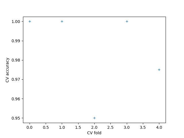
Shapelet forest embedding with LR
This example shows how to compute a shapelet forest embedding for a univariate time series dataset and use a logistic regression model to classify new samples
import matplotlib.pyplot as plt

from sklearn.linear_model import LogisticRegression
from sklearn.model_selection import cross_validate
from sklearn.pipeline import make_pipeline

from wildboar.datasets import load_dataset
from wildboar.ensemble import ShapeletForestEmbedding

random_state = 1234
x, y = load_dataset("GunPoint")

pipe = make_pipeline(
    ShapeletForestEmbedding(
        n_shapelets=1,
        min_shapelet_size=0,
        max_shapelet_size=1,
        metric="scaled_euclidean",
        sparse_output=True,
        max_depth=5,
        random_state=random_state,
        n_jobs=-1,
    ),
    LogisticRegression(solver="newton-cg", random_state=random_state),
)
cv = cross_validate(pipe, x, y, cv=5, scoring="accuracy", n_jobs=1)
plt.plot(cv["test_score"], linestyle="", marker="+")
plt.xlabel("CV fold")
plt.ylabel("CV accuracy")
plt.savefig("../fig/sfe_lr.png")
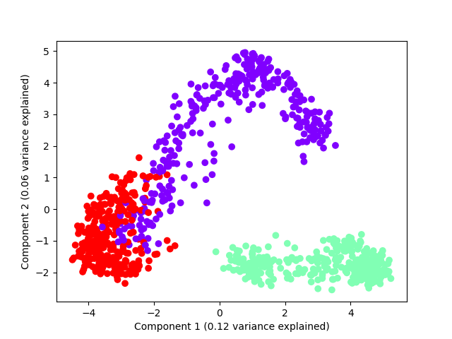
Shapelet forest embedding with PCA
This example shows how PCA can be used to plot the resulting embedding
import numpy as np
import matplotlib.pyplot as plt
from sklearn.decomposition import PCA

from sklearn.pipeline import make_pipeline

from wildboar.datasets import load_dataset
from wildboar.ensemble import ShapeletForestEmbedding

random_state = 1234
x, y = load_dataset("CBF")

pca = make_pipeline(
    ShapeletForestEmbedding(
        metric="scaled_euclidean",
        sparse_output=False,
        max_depth=5,
        random_state=random_state,
    ),
    PCA(n_components=2, random_state=random_state),
)
p = pca.fit_transform(x)
var = pca.steps[1][1].explained_variance_ratio_

labels, index = np.unique(y, return_inverse=True)
colors = plt.cm.rainbow(np.linspace(0, 1, len(labels)))
plt.scatter(p[:, 0], p[:, 1], color=colors[index, :])
plt.xlabel("Component 1 (%.2f variance explained)" % var[0])
plt.ylabel("Component 2 (%.2f variance explained)" % var[1])
plt.savefig("fig/sfe_pca.png")